Arrival time survey analysis

One of the courses in the sixth and final block of coursework in the MDS program is Experimentation and Causal Inference. In this class I was part of a small team who designed a survey to answer one specific and testable question.
Survey question
How does a student’s distance from campus influence arrival time to lectures?
We conducted an observational study to explore if there is a relationship between the distance lived from class and arrival time. We also wanted to test a potential confounder for this relationship which is the mode of transportation a student takes to class.
Our survey targeted MDS students specifically and their distance from our lecture hall, Hugh Dempster Pavilion at UBC.
Methods
Survey study design
We asked our survey respondents to answer the following questions:
-
How far from Hugh Dempster do you live in kilometers via the mode of transport you use (a google maps link was provided to help with the distance estimation)?
-
What time do you typically arrive at Hugh Dempster on Mondays and Wednesdays?
-
What time do you typically arrive at Hugh Dempster on Tuesdays and Thursdays?
-
What is your typical mode of transit? (multiple choice options: drive, public transit, walk, or bike)
Data collection methods
Data was collected via an online survey hosted by Qualtrics. The survey had 56 participants from the MDS students 2018-2019 cohort and responses were anonymized.
Analysis methods
We performed initial exploratory data analysis (EDA) on our data.
To analyze the data, we considered 3 groups:
-
All days grouped together
-
Mondays and Wednesdays together
-
Tuesdays and Thursdays together
Below we fit a linear regression using the distance as the predictor variable and the arrival time as the response variable. We compare this linear regression model with a null model through an ANOVA test. To validate the estimates of the frequentist approach, given the possibility of a small sample size, we use a Bayesian linear regression. After this, we will move on to using the mode of transportation as a confounder variable and fit a linear regression model with these variables. We will again validate the estimates using a Bayesian linear regression.
We used R for our work on this project.
Libraries
library(tidyverse)
library(tidybayes)
library(brms)
library(broom)
library(knitr)
library(gridExtra)
Load the data
clean_survey_all_days <- read_csv('https://raw.githubusercontent.com/rachelkriggs/rachelkriggs.github.io/master/data/arrival-time/clean_survey_responses_all_days.csv')
clean_survey_sep_days <- read_csv('https://raw.githubusercontent.com/rachelkriggs/rachelkriggs.github.io/master/data/arrival-time/clean_survey_responses_sep_days.csv')
EDA
plot1 <- clean_survey_all_days %>%
  ggplot() +
  geom_histogram(aes(x=distance_km)) +
  theme(axis.title=element_text(size=10),
        plot.title = element_text(size = 10, face = "bold")) +
  labs(y= "Frequency", x = "Distance (km)", title = "Distribution of Distance Lived From Campus (km)")

plot2 <- clean_survey_all_days %>%
  ggplot() +
  geom_histogram(aes(x=arrival)) +
  theme(axis.title=element_text(size=10),
        plot.title = element_text(size = 10, face = "bold")) +
  labs(y= "Frequency", x = "Arrival time (minutes)", title = "Distribution of Arrival Time (minutes)")

grid.arrange(plot1, plot2, ncol=2)
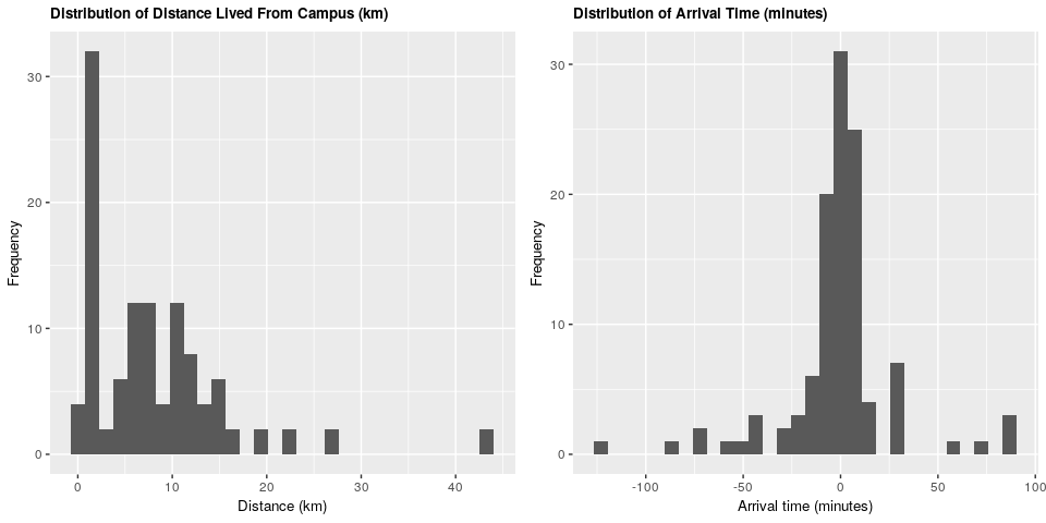
We can see that the majority of students live within 15 kilometers of campus, and that the majority arrive within 30 minutes before and 30 minutes after the start of the lecture.
plot3 <- clean_survey_all_days %>%
  ggplot() +
  geom_bar(aes(x=mode_of_transport)) +
  theme(axis.title=element_text(size=10),
        plot.title = element_text(size = 10, face = "bold")) +
  labs(y= "Frequency", x = "Mode of transport",
       title = "Number of MDS Students Using Different Modes of Transport")
plot3
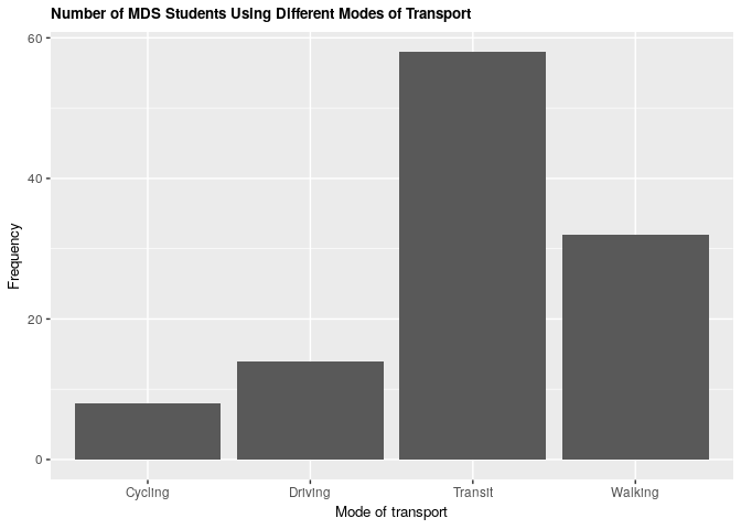
Comparing modes of transport, we see that public transit is the most common form of transportation, while cycling is the least.
Does there appear to be a relationship between arrival time and distance lived from campus? An initial plot shows us:
plot4 <- clean_survey_all_days %>%
  ggplot(aes(x = distance_km, y = arrival)) +
  geom_point() +
  theme(axis.title=element_text(size=10),
        plot.title = element_text(size = 10, face = "bold")) +
  labs(x = "Distance (km)", y = "Arrival time (minutes)",
       title = "Arrival Time vs Distance Lived From Campus",
       caption = "Negative arrival time numbers are interpreted as a student arrives early\nPositive arrival time numbers are interpreted as a student arrives late") +
  theme(plot.caption = element_text(face = "italic"))
plot4
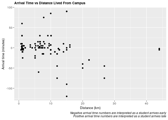
It’s difficult to discern from this plot so we will further explore this question in the analysis below.
plot5 <- clean_survey_sep_days %>%
  ggplot(aes(x = mw_arrival)) +
  geom_density(aes(fill = "salmon", color = "salmon"), alpha = .3) +
  geom_density(aes(x = tt_arrival, fill = "#00BFC4", color = "#00BFC4"), alpha = .3) +
  facet_wrap(~ mode_of_transport) +
  theme(axis.title=element_text(size=10),
        plot.title = element_text(size = 10, face = "bold")) +
  labs(x="Arrival Time (minutes)", y="Frequency", title = "Density of Student Arrival Time on Mon & Wed vs Tues & Thurs") +
  guides(color = FALSE) +
  scale_fill_identity(name = "days",
                      breaks = c("salmon", "#00BFC4"),
                      labels = c("Mon-Wed", "Tues-Thurs"),
                      guide = "legend")
plot5
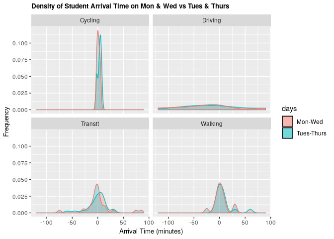
Comparing this distribution of arrival times on Mondays and Wednesdays vs Tuesdays and Thursdays reveals that there is only a slight difference in arrival time when the lecture starts at 09:00 (M-W) compared to when the lecture starts at 09:30 (Tu-Th). It is most noticeable for students taking transit.
Analysis and Results
The analysis is broken down as follows:
- Without Confounders
- 1.1.1 All days - Frequentist approach
- 1.1.2 All days - Bayesian validation
- 1.1.3 All days - Null model ANOVA test
- 1.2.1 Mon & Wed - Frequentist approach
- 1.2.2 Mon & Wed - Bayesian validation
- 1.2.3 Mon & Wed - Null model ANOVA test
- 1.3.1 Tues & Thurs - Frequentist approach
- 1.3.2 Tues & Thurs - Bayesian validation
- 1.3.3 Tues & Thurs - Null model ANOVA test
- With Confounders
- 2.1.1 All days - Frequentist approach
- 2.1.2 All days - Bayesian validation
- 2.2.1 Mon & Wed - Frequentist approach
- 2.2.2 Mon & Wed - Bayesian validation
- 2.3.1 Tues & Thurs - Frequentist approach
- 2.3.2 Tues & Thurs - Bayesian validation
- Results
1. Without Confounders
1.1 Distance and Arrival Time (All Days)
1.1.1 Frequentist approach
# Fit the frequentist model
fit_all <- lm(arrival ~ distance_km, data = clean_survey_all_days)

# Return the 95% estimates
tidy(fit_all) %>%
    bind_cols(confint_tidy(fit_all, conf.level = 0.95)) %>%
    select(term, estimate, conf.low, conf.high, p.value) %>%
    kable()
| term | estimate | conf.low | conf.high | p.value |
|---|---|---|---|---|
| (Intercept) | 6.7567108 | -0.8459198 | 14.3593413 | 0.0809729 |
| distance_km | -0.9445517 | -1.6316222 | -0.2574813 | 0.0074945 |
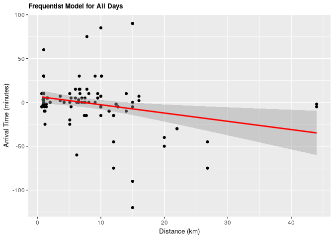
# Plot the frequentist model
ggplot(clean_survey_all_days, aes(x = distance_km, y = arrival)) +
  geom_point() +
  xlab("Distance (km)") +
  ylab("Arrival Time (minutes)") +
  ggtitle("Frequentist Model for All Days") +
  theme(axis.title=element_text(size=10),
        plot.title = element_text(size = 10, face = "bold")) +
  stat_smooth(method = "lm",
              col = "red")
1.1.2 Bayesian validation
# Fit the Bayesian model
fit_all_bayes <- brm(arrival ~ distance_km, data = clean_survey_all_days, iter = 5000, cores = -1)
# Return the 95% estimates
fit_all_bayes %>%
    gather_draws(b_Intercept, b_distance_km) %>%
    median_qi() %>%
    select(.variable, .value, .lower, .upper) %>%
    kable()
| .variable | .value | .lower | .upper |
|---|---|---|---|
| b_distance_km | -0.9474609 | -1.6336851 | -0.2606507 |
| b_Intercept | 6.8524700 | -0.4936192 | 14.2398776 |
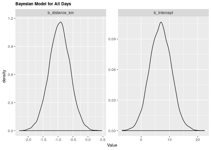
# Plot the Bayesian model
fit_all_bayes %>%
    gather_draws(b_Intercept, b_distance_km) %>%
    ggplot(aes(.value)) +
    geom_density() +
    facet_wrap(~ .variable, scales = 'free') +
    theme(axis.title=element_text(size=10),
          plot.title = element_text(size = 10, face = "bold")) +
    labs(x = 'Value',
         title = 'Bayesian Model for All Days')
1.1.3 ANOVA
# Anova

# Null model
fit_null_all <- lm(arrival ~ 1, data = clean_survey_all_days)

anova(fit_null_all, fit_all) %>% knitr::kable()
| Res.Df | RSS | Df | Sum of Sq | F | Pr(>F) |
|---|---|---|---|---|---|
| 111 | 92516.28 | NA | NA | NA | NA |
| 110 | 86668.11 | 1 | 5848.17 | 7.422554 | 0.0074945 |
Under both frequentist and Bayesian approaches there is an association between distance and arrival time. For the frequentist approach the estimate is -0.945 with a confidence interval of 95% (-1.604, -0.257). For the Bayesian approach the estimate is -0.949 with credible interval of 95% (-1.639, -0.267). As we can see from our ANOVA results, our model does significantly better than a null model, meaning that there is a significant explanatory power in adding distance from campus to explain to arrival time at the lecture hall.
For every increase of 1 km lived from campus, the expected change in arrival time is early by almost 1 minute.
1.2 Distance and Arrival Time (Monday & Wednesday)
1.2.1 Frequentist approach
fit_mw <- lm(mw_arrival ~ distance_km, data = clean_survey_sep_days)

tidy(fit_mw) %>%
    bind_cols(confint_tidy(fit_mw, conf.level = 0.95)) %>%
    select(term, estimate, conf.low, conf.high, p.value) %>%
    kable()
| term | estimate | conf.low | conf.high | p.value |
|---|---|---|---|---|
| (Intercept) | 6.8203611 | -3.030243 | 16.6709649 | 0.1707956 |
| distance_km | -0.8732192 | -1.763445 | 0.0170068 | 0.0543802 |
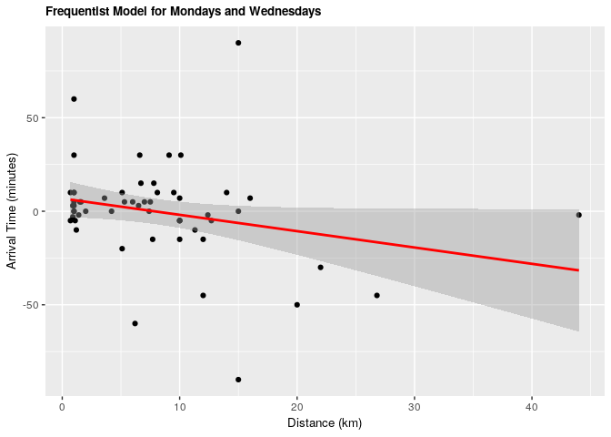
ggplot(clean_survey_sep_days, aes(x = distance_km, y = mw_arrival)) +
    geom_point() +
    ylab("Arrival Time (minutes)") +
    xlab("Distance (km)") +
    ggtitle("Frequentist Model for Mondays and Wednesdays") +
    theme(axis.title=element_text(size=10),
          plot.title = element_text(size = 10, face = "bold")) +
    stat_smooth(method = "lm", col = "red")
 1.2.2 Bayesian validation
fit_mw_bayes <- brm(mw_arrival ~ distance_km, data = clean_survey_sep_days, iter = 5000, cores = -1)
fit_mw_bayes %>%
    gather_draws(b_Intercept, b_distance_km) %>%
    median_qi() %>%
    select(.variable, .value, .lower, .upper) %>%
    kable()
| .variable | .value | .lower | .upper |
|---|---|---|---|
| b_distance_km | -0.8698122 | -1.736186 | 0.0056727 |
| b_Intercept | 7.0975600 | -2.273169 | 16.4472010 |
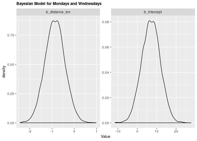
fit_mw_bayes %>%
    gather_draws(b_Intercept, b_distance_km) %>%
    ggplot(aes(.value)) +
    geom_density() +
    facet_wrap(~ .variable, scales = 'free') +
    theme(axis.title=element_text(size=10),
          plot.title = element_text(size = 10, face = "bold")) +
    labs(x = 'Value',
         title = 'Bayesian Model for Mondays and Wednesdays')
1.2.3 ANOVA
# Anova

# Null model
fit_null_mw <- lm(mw_arrival ~ 1, data = clean_survey_sep_days)

anova(fit_null_mw, fit_mw) %>% knitr::kable()
| Res.Df | RSS | Df | Sum of Sq | F | Pr(>F) |
|---|---|---|---|---|---|
| 55 | 37393.55 | NA | NA | NA | NA |
| 54 | 34894.45 | 1 | 2499.108 | 3.86743 | 0.0543802 |
Under both frequentist and Bayesian approaches there is not an association between distance and arrival time for Mondays and Wednesdays. For the frequentist approach the estimate is -0.87 with a confidence interval of 95% (-1.76, 0.01). For the Bayesian approach the estimate is -0.87 with credible interval of 95% (-1.75, 0.01). As we can see from our ANOVA results, our model doesn’t do significantly better than a null model, meaning that there is no significant explanatory power in adding distance from campus to explain to arrival time at the lecture hall for Mondays and Wednesdays.
1.3 Distance and Arrival Time (Tuesday & Thursday)
1.3.1 Frequentist approach
fit_tt <- lm(tt_arrival ~ distance_km, data = clean_survey_sep_days)

tidy(fit_tt) %>%
    bind_cols(confint_tidy(fit_tt, conf.level = 0.95)) %>%
    select(term, estimate, conf.low, conf.high, p.value) %>%
    kable()
| term | estimate | conf.low | conf.high | p.value |
|---|---|---|---|---|
| (Intercept) | 6.693060 | -5.296692 | 18.6828132 | 0.2680140 |
| distance_km | -1.015884 | -2.099431 | 0.0676624 | 0.0655509 |
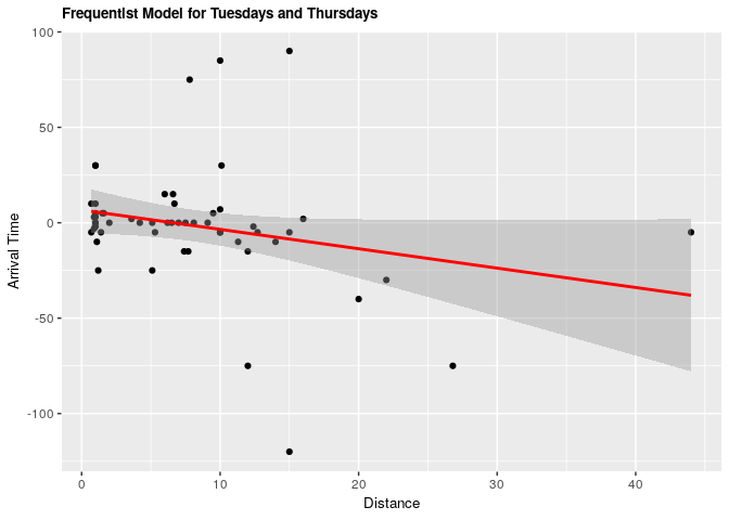
ggplot(clean_survey_sep_days, aes(x = distance_km, y = tt_arrival)) +
    geom_point() +
    ylab("Arrival Time") +
    xlab("Distance") +
    ggtitle("Frequentist Model for Tuesdays and Thursdays") +
    theme(axis.title=element_text(size=10),
          plot.title = element_text(size = 10, face = "bold")) +
    stat_smooth(method = "lm", col = "red")
1.3.2 Bayesian validation
fit_tt_bayes <- brm(tt_arrival ~ distance_km, data = clean_survey_sep_days, iter = 5000, cores = -1)
fit_tt_bayes %>%
    gather_draws(b_Intercept, b_distance_km) %>%
    median_qi() %>%
    select(.variable, .value, .lower, .upper) %>%
    kable()
| .variable | .value | .lower | .upper |
|---|---|---|---|
| b_distance_km | -1.027198 | -2.080223 | -0.0072312 |
| b_Intercept | 6.909039 | -4.098512 | 18.2462742 |
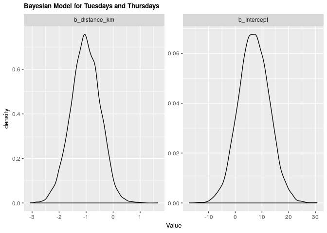
fit_tt_bayes %>%
    gather_draws(b_Intercept, b_distance_km) %>%
    ggplot(aes(.value)) +
    geom_density() +
    facet_wrap(~ .variable, scales = 'free') +
    theme(axis.title=element_text(size=10),
          plot.title = element_text(size = 10, face = "bold")) +
    labs(x = 'Value',
         title = 'Bayesian Model for Tuesdays and Thursdays')
1.3.3 ANOVA
# Anova

# Null model
fit_null_tt <- lm(tt_arrival ~ 1, data = clean_survey_sep_days)

anova(fit_null_tt, fit_tt) %>% knitr::kable()
| Res.Df | RSS | Df | Sum of Sq | F | Pr(>F) |
|---|---|---|---|---|---|
| 55 | 55077.71 | NA | NA | NA | NA |
| 54 | 51695.30 | 1 | 3382.416 | 3.533212 | 0.0655509 |
Under both frequentist and Bayesian approaches there is not an association between distance and arrival time for Tuesdays and Thursdays. For the frequentist approach the estimate is -1.02 with a confidence interval of 95% (-2.1, 0.0677). For the Bayesian approach the estimate is -1.02 with credible interval of 95% (-2.05, 0.02). As we can see from our ANOVA results, our model does not do significantly better than a null model, meaning that there is no significant explanatory power in adding distance from campus to explain to arrival time at the lecture hall for Tuesdays and Thursdays.
2. With Confounders
2.1 Distance and Arrival Time (All Days)
2.1.1 Frequentist approach
fit_all_transp <- lm(arrival ~ distance_km + mode_of_transport, data = clean_survey_all_days)
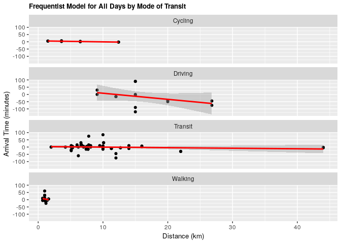
ggplot(clean_survey_all_days, aes(x = distance_km, y = arrival)) +
    geom_point() +
    ylab("Arrival Time (minutes)") +
    xlab("Distance (km)") +
    ggtitle("Frequentist Model for All Days by Mode of Transit") +
    facet_wrap(~ mode_of_transport, nrow = 4) +
    theme(axis.title=element_text(size=10),
          plot.title = element_text(size = 10, face = "bold")) +
    geom_smooth(method = 'lm', col = 'red')
2.1.2 Bayesian validation
fit_all_bayes_transp <- brm(arrival ~ distance_km + mode_of_transport, data = clean_survey_all_days, iter = 5000, cores = -1)
fit_all_bayes_transp%>%
    gather_draws(b_Intercept, b_distance_km, b_mode_of_transportDriving, b_mode_of_transportTransit, b_mode_of_transportWalking) %>%
    ggplot(aes(.value)) +
    geom_density() +
    facet_wrap(~ .variable, scales = 'free') +
    labs(x = 'Value',
         title = 'Bayesian Model for All Days by Mode of Transit') +
    theme(axis.title=element_text(size=10),
          plot.title = element_text(size = 10, face = "bold"))
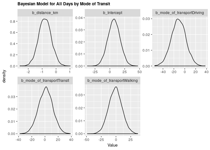
Under both frequentist and Bayesian approaches there is an association between distance and arrival time when including confounders. We can compare the two estimates in the tables below:
Frequentist
tidy(fit_all_transp) %>%
    bind_cols(confint_tidy(fit_all_transp, conf.level = 0.95)) %>%
    select(term, estimate, conf.low, conf.high, p.value) %>%
    kable()
| term | estimate | conf.low | conf.high | p.value |
|---|---|---|---|---|
| (Intercept) | 7.0621190 | -13.438025 | 27.5622628 | 0.4961374 |
| distance_km | -0.8020198 | -1.711544 | 0.1075044 | 0.0833205 |
| mode_of_transportDriving | -11.6266849 | -38.055241 | 14.8018711 | 0.3851024 |
| mode_of_transportTransit | 0.7494133 | -20.664819 | 22.1636458 | 0.9448202 |
| mode_of_transportWalking | -1.3287860 | -23.879118 | 21.2215461 | 0.9072275 |
Bayesian
fit_all_bayes_transp  %>%
    gather_draws(b_Intercept, b_distance_km, b_mode_of_transportDriving, b_mode_of_transportTransit, b_mode_of_transportWalking) %>%
    median_qi() %>%
    select(.variable, .value, .lower, .upper) %>%
    kable()
| .variable | .value | .lower | .upper |
|---|---|---|---|
| b_distance_km | -0.8063163 | -1.708165 | 0.0962294 |
| b_Intercept | 7.0174746 | -13.211175 | 26.8852943 |
| b_mode_of_transportDriving | -11.4761765 | -37.536480 | 14.5129933 |
| b_mode_of_transportTransit | 1.0980724 | -20.558743 | 22.1344916 |
| b_mode_of_transportWalking | -1.0413373 | -23.098937 | 21.2279271 |
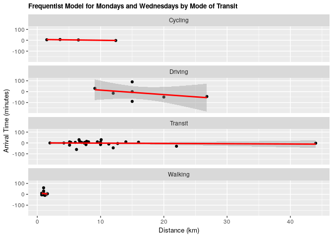
2.2 Distance and Arrival Time (Monday & Wednesday)
2.2.1 Frequentist approach
fit_mw_transp <- lm(mw_arrival ~ distance_km + mode_of_transport, data = clean_survey_sep_days)
ggplot(clean_survey_sep_days, aes(x = distance_km, y = mw_arrival)) +
    geom_point() +
    ylab("Arrival Time (minutes)") +
    xlab("Distance (km)") +
    ggtitle("Frequentist Model for Mondays and Wednesdays by Mode of Transit") +
    theme(axis.title=element_text(size=10),
          plot.title = element_text(size = 10, face = "bold")) +
    facet_wrap(~ mode_of_transport, nrow = 4) +
    geom_smooth(method = 'lm', col = 'red')
2.2.2 Bayesian validation
fit_mw_bayes_transp <- brm(mw_arrival ~ distance_km + mode_of_transport, data = clean_survey_sep_days, iter = 5000, cores = -1)
fit_mw_bayes_transp %>%
    gather_draws(b_Intercept, b_distance_km, b_mode_of_transportDriving,
                 b_mode_of_transportTransit, b_mode_of_transportWalking) %>%
    ggplot(aes(.value)) +
    geom_density() +
    facet_wrap(~ .variable, scales = 'free') +
    labs(x = 'Value',
         title = 'Bayesian Model for Mondays and Wednesdays by Mode of Transit') +
    theme(axis.title=element_text(size=10),
          plot.title = element_text(size = 10, face = "bold"))
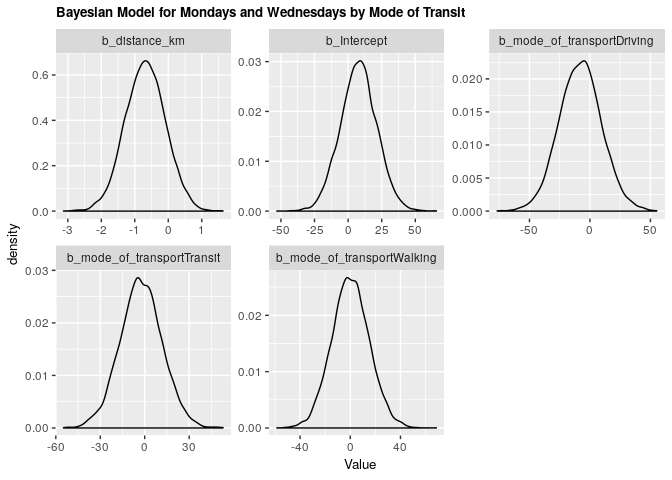
Under both frequentist and Bayesian approaches there is an association between distance and arrival time for Monday & Wednesday when including confounders. We can compare the two estimates in the tables below:
Frequentist
tidy(fit_mw_transp)%>%
    bind_cols(confint_tidy(fit_mw_transp, conf.level = 0.95)) %>%
    select(term, estimate, conf.low, conf.high, p.value) %>%
    kable()
| term | estimate | conf.low | conf.high | p.value |
|---|---|---|---|---|
| (Intercept) | 7.3754923 | -19.779601 | 34.5305861 | 0.5879432 |
| distance_km | -0.6875821 | -1.892365 | 0.5172004 | 0.2572468 |
| mode_of_transportDriving | -7.7143475 | -42.722391 | 27.2936955 | 0.6600777 |
| mode_of_transportTransit | -2.2253062 | -30.591229 | 26.1406164 | 0.8754767 |
| mode_of_transportWalking | 0.2710767 | -29.599757 | 30.1419103 | 0.9855354 |
Bayesian
fit_mw_bayes_transp %>%
    gather_draws(b_Intercept, b_distance_km, b_mode_of_transportDriving,
                 b_mode_of_transportTransit, b_mode_of_transportWalking) %>%
    median_qi() %>%
    select(.variable, .value, .lower, .upper) %>%
    kable()
| .variable | .value | .lower | .upper |
|---|---|---|---|
| b_distance_km | -0.6813593 | -1.865392 | 0.4916241 |
| b_Intercept | 7.8496529 | -19.095773 | 34.5034738 |
| b_mode_of_transportDriving | -7.9289231 | -42.256181 | 27.0616609 |
| b_mode_of_transportTransit | -2.5916423 | -30.811485 | 25.9093391 |
| b_mode_of_transportWalking | 0.0414775 | -28.709157 | 29.7268700 |
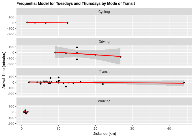
2.3 Distance and Arrival Time (Tuesday & Thursday)
2.3.1 Frequentist approach
fit_tt_transp <- lm(tt_arrival ~ distance_km + mode_of_transport, data = clean_survey_sep_days)
ggplot(clean_survey_sep_days, aes(x = distance_km, y = tt_arrival)) +
    geom_point() +
    ylab("Arrival Time (minutes)") +
    xlab("Distance (km)") +
    ggtitle("Frequentist Model for Tuesdays and Thursdays by Mode of Transit") +
    theme(axis.title=element_text(size=10),
          plot.title = element_text(size = 10, face = "bold")) +
    facet_wrap(~ mode_of_transport, nrow = 4) +
    geom_smooth(method = 'lm', col = 'red')
2.3.2 Bayesian validation
fit_tt_bayes_transp <- brm(tt_arrival ~ distance_km + mode_of_transport, data = clean_survey_sep_days, iter = 5000, cores = -1)
fit_tt_bayes_transp %>%
    gather_draws(b_Intercept, b_distance_km, b_mode_of_transportDriving, b_mode_of_transportTransit, b_mode_of_transportWalking) %>%
    ggplot(aes(.value)) +
    geom_density() +
    facet_wrap(~ .variable, scales = 'free') +
    labs(x = 'Value',
         title = 'Bayesian Model for Tuesdays and Thursdays by Mode of Transit') +
    theme(axis.title=element_text(size=10),
          plot.title = element_text(size = 10, face = "bold"))
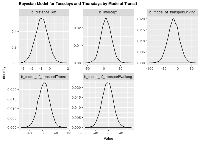
Under both frequentist and Bayesian approaches there is an association between distance and arrival time for Tuesdays and Thursdays when including confounders. We can compare the two estimates in the tables below:
Frequentist
tidy(fit_tt_transp)%>%
    bind_cols(confint_tidy(fit_tt_transp, conf.level = 0.95)) %>%
    select(term, estimate, conf.low, conf.high, p.value) %>%
    kable()
| term | estimate | conf.low | conf.high | p.value |
|---|---|---|---|---|
| (Intercept) | 6.7487456 | -25.706900 | 39.204391 | 0.6781001 |
| distance_km | -0.9164576 | -2.356408 | 0.523493 | 0.2071309 |
| mode_of_transportDriving | -15.5390222 | -57.380478 | 26.302433 | 0.4593476 |
| mode_of_transportTransit | 3.7241328 | -30.178690 | 37.626956 | 0.8263407 |
| mode_of_transportWalking | -2.9286487 | -38.630135 | 32.772837 | 0.8698427 |
Bayesian
fit_tt_bayes_transp %>%
    gather_draws(b_Intercept, b_distance_km, b_mode_of_transportDriving,
                 b_mode_of_transportTransit, b_mode_of_transportWalking) %>%
    median_qi() %>%
    select(.variable, .value, .lower, .upper) %>%
    kable()
| .variable | .value | .lower | .upper |
|---|---|---|---|
| b_distance_km | -0.9286238 | -2.33724 | 0.4455929 |
| b_Intercept | 6.7594665 | -24.23578 | 39.2244426 |
| b_mode_of_transportDriving | -15.1856723 | -55.73532 | 25.5966720 |
| b_mode_of_transportTransit | 4.1427389 | -29.59664 | 36.5537388 |
| b_mode_of_transportWalking | -2.5655778 | -37.70048 | 31.9125465 |
3. Results
From our results we can see that there is a relationship between how far someone lives from campus and their arrival time. This was found for all days overall and for the two groups of days (Mondays-Wednesdays, Tuesdays-Thursdays). Given the consistency between methods in both the estimates achieved and the confidence/credible intervals allows us to infer that there is an association between how far someone lives from campus and their time of arrival. However, when comparing the frequentist models to a null model, only the overall model did significantly better than the null model. This might be explained by Simpson’s paradox. This picture changed when including mode of transport as our confounder in the analysis. When doing this component, we observed that mode of transport does not have an effect as a confounder as our estimates did not change to be outside of the confidence/credible intervals of the first estimates. This phenomena remained both for the overall analysis and for the focused analysis in the groups of days.
Collaborators on this project include myself, Ian Flores Siaca, Akansha Vashisth, and Milos Milic.
Photo by Andrik Langfield on Unsplash